Control Chart

A control chart is a graphical display of a measure of a quality characteristic (weight, length, temperature, waiting time, etc.) over time. The measurement of the characteristic is plotted on the vertical axis, with the sample number (also called subgroup, subsample, or just sample number) on the horizontal axis. The time that the sample was taken should also be recorded so that the sample number can give information to the operator and management about problems as they occur. A central value—the process mean—is usually plotted as a horizontal solid line and upper and lower control limits as horizontal dotted lines.

A control chart provides a visual representation of some process metric, with an emphasis on variation in that metric. All processes will have some degree of variation, but if that variation is within acceptable limits, the process can still be described as “stable” or “in control.” The goal of using a control chart is to achieve and maintain stability – keeping the process consistently within acceptable parameters, and expected to remain consistent in the future.

What is a Control Chart?

There are a number of different types of control charts. This example will focus on a simple form called a univariate control chart, which measures a single changing variable.

A control chart shows the value of a measured quality characteristic over a period of time, or through a series of samples. A quality characteristic is something measurable, such as weight, length, brightness, temperature, delivery time, or another similar characteristic.

The mean, or average, value for the chosen characteristic is determined and plotted horizontally on a chart. This is the center line. Then two other lines are placed on the chart: an Upper Control Limit (UCL) and a Lower Control Limit (LCL). These are located at points above and below the mean, determined by statistical rules. The measured values are then marked on the control chart, and problems or trends can be easily seen.

Often, a control chart will show two graphs. The first chart will appear as described above, comparing the measured values (or an average of several measured values) to a target value. On its own, this may not be enough information, though. For example, if the desired length of a widget is 15 cm, and three measured values are 17, 15, and 13 cm, then on average the desired length is being produced. However, this process clearly has a problem: while the average is good, the process is not consistent. This is where the second graph will come in.

The second graph on a common control chart shows the range of measured values — how closely grouped or widely spread the measurements are, compared to each other. In the example above, a wide range of lengths is being produced, and this chart would show that as a high variation; the process is not stable. However, if the three widget lengths were 15.01, 15.00, and 14.99 cm, then the measurements would have a much smaller range. This would be a stable process. The addition of the second graph to the control chart allows both aspects of quality to be shown.

Control Chart – Calculating the Mean, UCL, and LCL

A control chart starts with a decision on the characteristic to be measured, and the collection of the data pertaining to that measurement. For this example, we’ll look at the length of widgets being made in a factory. The length of five widgets is measured at the beginning of each hour for ten hours. We'll then have a table of length data:

	8:00 AM	9:00 AM	10:00 AM	11:00 AM	12:00 PM	1:00 PM	2:00 PM	3:00 PM	4:00 PM	5:00 PM
1	14.3	15	14.7	16.5	14.9	14.1	14.1	15.3	14.8	16
2	15.2	14.3	15	15.8	15.4	14.4	15.1	16.4	15.9	15.9
3	15.1	15.6	13.6	16.2	17.4	15.1	16.5	13.6	15.2	15.5
4	14.4	15.6	13.7	14.7	15.5	15.3	16.1	14.7	14.5	14.2
5	16.4	14.8	14.5	15.1	15.5	17.9	14.5	15.4	15.1	15.7

The next step is to calculate the mean, or average, of each set of measurements. Add the values in the column and divide by the number of values, in this case five. Here, another row has been added to show the mean for each column.

	8:00 AM	9:00 AM	10:00 AM	11:00 AM	12:00 PM	1:00 PM	2:00 PM	3:00 PM	4:00 PM	5:00 PM
1	14.3	15	14.7	16.5	14.9	16.1	14.1	15.3	14.8	16
2	15.2	14.3	15	15.8	15.4	14.4	15.1	16.4	15.9	15.9
3	15.1	15.6	13.6	16.2	17.4	15.1	14.5	13.6	15.2	15.5
4	14.4	15.6	13.7	14.7	15.5	15.3	14.1	14.7	14.5	14.2
5	16.4	14.8	14.5	15.1	15.5	17.9	13.9	15.4	15.1	15.7
Mean	15.08	15.06	14.3	15.66	15.74	15.76	14.34	15.08	15.16	15.46

 

Using the calculated mean values, we then calculate the “grand mean,” or the mean of the mean values. Thus we add all of the means together and divide by ten. In this example, that would be:

(15.08+15.06+14.3+15.66+15.74+15.76+14.34+15.08+15.16+15.46)/10 = 15.16

This grand mean (15.16) will be the center line of the first graph (the length graph) in our control chart.

For the second graph (the range graph), we'll need to calculate the range for each set of measurements. The range equals the largest value in each set minus the smallest value in that set; for example, the 8:00 AM measurements range from 16.4 to 14.3, so the range for that hour is 2.1. The range for each sample has been added to the chart below.

	8:00 AM	9:00 AM	10:00 AM	11:00 AM	12:00 PM	1:00 PM	2:00 PM	3:00 PM	4:00 PM	5:00 PM
1	14.3	15	14.7	16.5	14.9	16.1	14.1	15.3	14.8	16
2	15.2	14.3	15	15.8	15.4	14.4	15.1	16.4	15.9	15.9
3	15.1	15.6	13.6	16.2	17.4	15.1	14.5	13.6	15.2	15.5
4	14.4	15.6	13.7	14.7	15.5	15.3	14.1	14.7	14.5	14.2
5	16.4	14.8	14.5	15.1	15.5	17.9	13.9	15.4	15.1	15.7
Mean	15.08	15.06	14.3	15.66	15.74	15.76	14.34	15.08	15.16	15.46
Range	2.1	0.7	1.4	1.5	2	3.5	1.2	2.8	1.4	1.7

Next, calculate the mean of the ranges. This will become the center line of the second graph on the control chart.

(2.1+0.7+1.4+1.5+2.0+3.5+1.2+2.8+1.4+1.7)/10 = 1.83

A table of constants, reproduced here, is used to calculate the UCL and LCL for the length and range graphs. There is a different adjuster for the Limits of each graph; the number “n” is the number of samples in each set (in our example, the measurements taken per hour: five).

n (Number of Samples)	A (Measurement Limit Adjuster)	D (Range Limit Adjuster)
2	1.880	3.267
3	1.023	2.574
4	0.729	2.282
5	0.577	2.114
6	0.483	2.004
7	0.419	1.924
8	0.373	1.864
9	0.337	1.816
10	0.308	1.777
11	0.285	1.744
12	0.266	1.717
13	0.249	1.693
14	0.235	1.672
15	0.223	1.653

For the length graph, the Upper and Lower Control Limits (UCL and LCL) are calculated with the following formulas:

UCL = (Grand Mean) + (A)(Mean of Ranges) = 15.16 + (0.577)(1.83) = 16.22

LCL = (Grand Mean) - (A)(Mean of Ranges) = 15.16 - (0.577)(1.83) = 14.10

For the range graph, the Upper Control Limit (UCL) is calculated with this formula:

UCL = (D)(Average of Ranges) = (2.114)(1.83) = 3.87

The range graph will have no Lower Control Limit — no minimum expected amount of variation — unless the sample sets include seven or more samples. Our example will only need one calculated limit for the range graph.

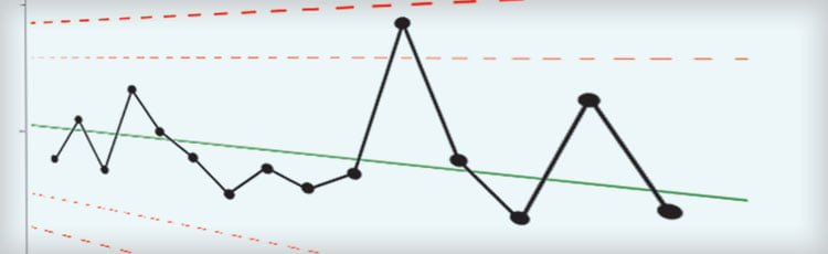
Now that we have the calculations done, we can draw the graphs. In this example, the center lines (the mean length and mean range) have been drawn as solid lines, and the Upper and Lower Control Limits have been drawn as dashed lines.

Two other horizontal lines (gray, in this example) have been added to the graphs. These are the “1-sigma” and “2-sigma” lines, placed by evenly dividing the space between the center line and the UCL or LCL (which are, in effect, “3-sigma” lines.) Each sigma represents a level of variation, and the way in which the plotted points fall above or below those lines will provide information about the trends in variation.

Learn more about 5S by downloading your copy of our free 5S System Best Practices Guide below!